Confidence Interval-Based Estimation of Relevance (CIBER)
Source:R/CIBER.R, R/binaryCIBER.R, R/detStructCIBER.R
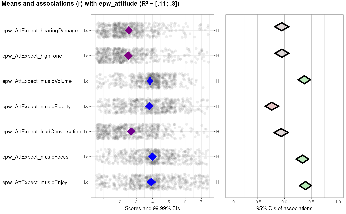
CIBER.RdThis function generates a high-level plot consisting of several diamond plots. This function is useful for estimating the relative relevance of a set of determinants of, for example, behavior. The plot in the left hand panel shows each determinant's distribution with a diamond representing the confidence interval. The right hand plot shows the determinants' associations to one or more 'target' variables, such as behavior or determinants of behavior.
CIBER(
  data,
  determinants,
  targets,
  conf.level = list(means = 0.9999, associations = 0.95),
  subQuestions = NULL,
  leftAnchors = rep("Lo", length(determinants)),
  rightAnchors = rep("Hi", length(determinants)),
  outputFile = NULL,
  outputWidth = NULL,
  outputHeight = NULL,
  outputUnits = "in",
  outputParams = list(),
  orderBy = NULL,
  decreasing = NULL,
  numberSubQuestions = FALSE,
  generateColors = list(means = c("red", "blue", "green"), associations = c("red",
    "grey", "green")),
  strokeColors = viridis::viridis(length(targets)),
  vLines = c(-0.5, 0, 0.5),
  vLineColors = "grey",
  titlePrefix = "Means and associations (r) with",
  titleVarLabels = NULL,
  titleSuffix = "",
  fullColorRange = NULL,
  associationsAlpha = 0.5,
  returnPlotOnly = TRUE,
  drawPlot = TRUE,
  jitterWidth = 0.45,
  baseSize = 0.8,
  dotSize = 2.5 * baseSize,
  baseFontSize = 10 * baseSize,
  theme = ggplot2::theme_bw(base_size = baseFontSize),
  xbreaks = NULL,
  rsq = TRUE,
  ...
)

binaryCIBER(
  data,
  determinants,
  targets,
  conf.level = list(means = 0.9999, associations = 0.95),
  subQuestions = NULL,
  leftAnchors = rep("Lo", length(determinants)),
  rightAnchors = rep("Hi", length(determinants)),
  outputFile = NULL,
  outputWidth = NULL,
  outputHeight = NULL,
  outputUnits = "in",
  outputParams = list(),
  orderBy = NULL,
  decreasing = NULL,
  numberSubQuestions = FALSE,
  comparisonColors = viridis::viridis(2, end = 0.5),
  categoryLabels = NULL,
  generateColors = list(means = c("red", "blue", "green"), associations = c("red",
    "grey", "green")),
  strokeColors = viridis::viridis(length(targets)),
  vLines = c(-0.8, 0, 0.8),
  vLineColors = "grey",
  titlePrefix = "Means and associations (d) with",
  titleVarLabels = NULL,
  titleSuffix = "",
  fullColorRange = NULL,
  associationsAlpha = 0.5,
  returnPlotOnly = TRUE,
  drawPlot = TRUE,
  baseSize = 0.8,
  dotSize = 2.5 * baseSize,
  baseFontSize = 10 * baseSize,
  theme = ggplot2::theme_bw(base_size = baseFontSize),
  xbreaks = NULL,
  ...
)

detStructCIBER(
  determinantStructure,
  data,
  conf.level = list(means = 0.9999, associations = 0.95),
  subQuestions = NULL,
  leftAnchors = rep("Lo", length(determinants)),
  rightAnchors = rep("Hi", length(determinants)),
  orderBy = 1,
  decreasing = NULL,
  generateColors = list(means = c("red", "blue", "green"), associations = c("red",
    "grey", "green")),
  strokeColors = NULL,
  titlePrefix = "Means and associations with",
  titleVarLabels = NULL,
  titleSuffix = "",
  fullColorRange = NULL,
  associationsAlpha = 0.5,
  baseSize = 0.8,
  dotSize = 2.5 * baseSize,
  baseFontSize = 10 * baseSize,
  theme = ggplot2::theme_bw(base_size = baseFontSize),
  ...
)
Arguments
- data
The dataframe containing the variables.
- determinants
The 'determinants': the predictors (or 'covariates') of the target variables(s) (or 'criteria').
- targets
The 'targets' or 'criteria' variables: the variables predicted by the determinants.
- conf.level
The confidence levels for the confidence intervals: has to be a named list with two elements:
meansandassociations, specifying the desired confidence levels for the means and associations, respectively. The confidence level for the associations is also used for the intervals for the proportions of explained variance.- subQuestions
The subquestions used to measure each determinants. This can also be used to provide pretty names for the variables if the determinants were not measured by one question each. Must have the same length as
determinants.- leftAnchors
The anchors to display on the left side of the left hand panel. If the determinants were measured with one variable each, this can be used to show the anchors that were used for the respective scales. Must have the same length as
determinants.- rightAnchors
The anchors to display on the left side of the left hand panel. If the determinants were measured with one variable each, this can be used to show the anchors that were used for the respective scales. Must have the same length as
determinants.- outputFile
The file to write the output to (the plot is not stored to disk if
NULL). The extension can be specified to change the file type.- outputWidth, outputHeight, outputUnits
The width, height, and units for the output file.
- outputParams
More advanced parameters for the output file. This can be used to pass arguments to
ggplot2::ggsave(), such as passingoutputParams=list(type="cairo-png")to use anti-aliasing when saving a PNG file.- orderBy
Whether to sort the determinants. Set to
NULLto not sort at all; specify the name or index of one of thetargets to sort by the point estimates of the associations with that target variable. Usedecreasingto determine whether to sort in ascending or descending order. For convenience, iforderByis notNULL, butdecreasingis, the determinants are sorted in descending (decreasing) order.- decreasing
Whether to sort the determinants. Specify
NULLto not sort at all,TRUEto sort in descending order, andFALSEto sort in ascending order. Ifdecreasingis norNULL, butorderByisNULL, the determinants are sorted by their means. For convenience, iforderByis notNULL, butdecreasingis, the determinants are sorted in descending (decreasing) order.- numberSubQuestions
Whether or not to number the subquestions. If they are numbered, they are numbered from the top to the bottom.
- generateColors
The colors to use to generate the gradients for coloring the diamonds representing the confidence intervals. Has to be a named list with two elements:
meansandassociations, specifying the desired colors for the means and associations, respectively.- strokeColors
The palette to use to color the stroke of the confidence intervals for the associations between the determinants and the targets. Successive colors from this palette are used for the targets.
- vLines, vLineColors
In the association plot, vertical lines can be plotted to facilitate interpretation. Specify their locations and colors here, or set one or both to
NULLto eliminate them.- titlePrefix
Text to add before the list of target names and the proportions of explained variance for each target. This plot title also serves as legend to indicate which target 'gets' which each color.
- titleVarLabels
Optionally, variable labels to use in the plot title. Has to be the exact same length as
targets.- titleSuffix
Text to add after the list of target names and the proportions of explained variance for each target.
- fullColorRange
If colors are specified, this can be used to specify which values, for the determinant confidence intervals in the left hand panel, are the minimum and maximum. This is useful if those scores are not actually in the data (e.g. for extremely skewed distributions). If
NULL, the range of all individual scores on the determinants is used. For the associations,c(-1, 1)is always used asfullColorRange.- associationsAlpha
The alpha level (transparency) of the confidence interval diamonds in the right hand plot. Value between 0 and 1, where 0 signifies complete transparency (i.e. invisibility) and 1 signifies complete 'opaqueness'.
- returnPlotOnly
Whether to return the entire object that is generated (including all intermediate objects) or only the plot.
- drawPlot
Whether the draw the plot, or only return it.
- jitterWidth
How much to jitter the data points in the left hand plot.
- baseSize
This can be used to efficiently change the size of most plot elements.
- dotSize
This is the size of the points used to show the individual data points in the left hand plot.
- baseFontSize
This can be used to set the font size separately from the
baseSize.- theme
This is the theme that is used for the plots.
- xbreaks
Which breaks to use on the X axis (can be useful to override
ggplot2's defaults).- rsq
Whether to compute the R squared values.
- ...
These arguments are passed on to
biAxisDiamondPlot(for the left panel) anddiamondPlot(for the right panel). Note that all argument are passed to both those functions.- comparisonColors
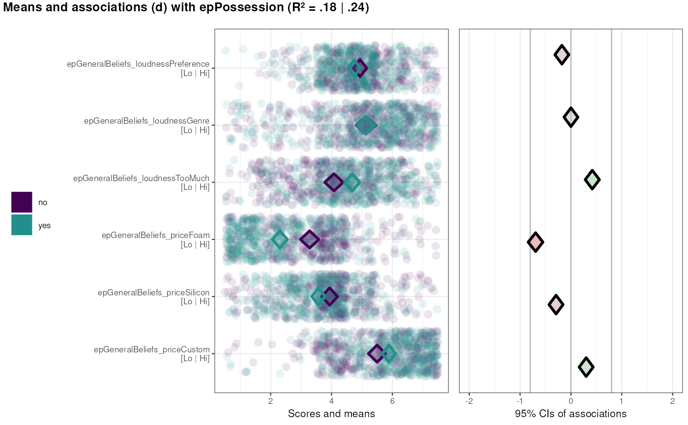
Colors to use for the two groups in a binary CIBER plot with one (dichotomous) target.
- categoryLabels
Labels for the two values of the target.
- determinantStructure
When using
detStructCIBER, the determinant structure as generated bydeterminantStructureis included here.determinants,targets,subQuestions,leftAnchors, andrightAnchorsare then read from thedeterminantStructureobject. In other words: once adeterminantStructurehas been generated, onlydatanddeterminantStructurehave to be provided as argument to generate a CIBER diamond plot.
Value
Depending on the value of returnPlotOnly, either the plot
only (a gtable object) or an object containing most objects
created along the way (in which case the plot is stored in
$output$plot).
The plot has width and height attributes which can be used
when saving the plot.
Details
Details are explained in Crutzen & Peters (2017).
References
Crutzen, R., Peters, G.-J. Y., & Noijen, J. (2017). How to Select Relevant Social-Cognitive Determinants and Use them in the Development of Behaviour Change Interventions? Confidence Interval-Based Estimation of Relevance. http://dx.doi.org/
See also
Examples
### This example uses the determinant study Party Panel 17.1;
### see ?behaviorchange::BBC_data for more information.
data(BBC_pp17.1);
behaviorchange::CIBER(data=BBC_pp17.1,
                      determinants=c('epw_AttExpect_hearingDamage',
                                     'epw_AttExpect_highTone',
                                     'epw_AttExpect_musicVolume',
                                     'epw_AttExpect_musicFidelity',
                                     'epw_AttExpect_loudConversation',
                                     'epw_AttExpect_musicFocus',
                                     'epw_AttExpect_musicEnjoy'),
                      targets=c('epw_attitude'));


### With a binary target
data(BBC_pp17.1);
behaviorchange::binaryCIBER(data=BBC_pp17.1,
                            determinants=c('epGeneralBeliefs_loudnessPreference',
                                           'epGeneralBeliefs_loudnessGenre',
                                           'epGeneralBeliefs_loudnessTooMuch',
                                           'epGeneralBeliefs_priceFoam',
                                           'epGeneralBeliefs_priceSilicon',
                                           'epGeneralBeliefs_priceCustom'),
                            targets=c('epPossession'),
                            categoryLabels = c('no',
                                               'yes'));
